Patriot Viper III Review: 2x4 GB at DDR3-2400 C10-12-12 1.65 V
by Ian Cutress on November 18, 2013 1:00 PM ESTCPU Compute
One side I like to exploit on CPUs is the ability to compute and whether a variety of mathematical loads can stress the system in a way that real-world usage might not. For these benchmarks we are ones developed for testing MP servers and workstation systems back in early 2013, such as grid solvers and Brownian motion code. Please head over to the first of such reviews where the mathematics and small snippets of code are available.
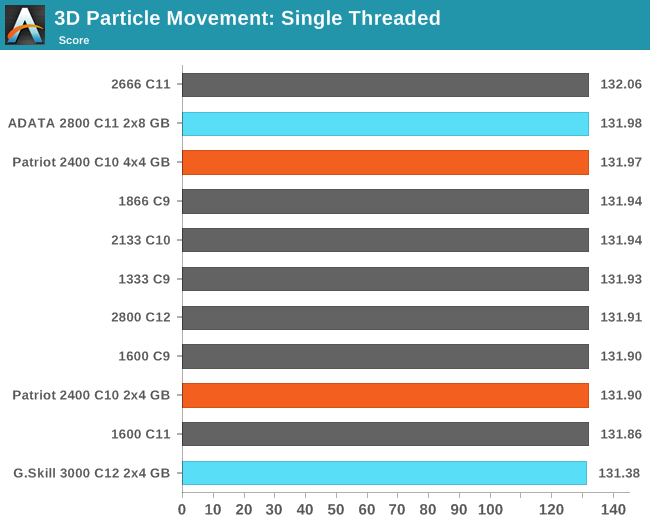
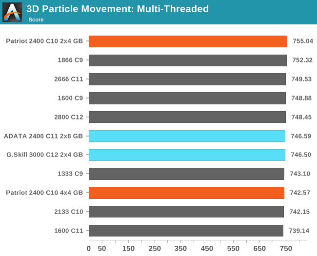
3D Movement Algorithm Test
The algorithms in 3DPM employ uniform random number generation or normal distribution random number generation, and vary in various amounts of trigonometric operations, conditional statements, generation and rejection, fused operations, etc. The benchmark runs through six algorithms for a specified number of particles and steps, and calculates the speed of each algorithm, then sums them all for a final score. This is an example of a real world situation that a computational scientist may find themselves in, rather than a pure synthetic benchmark. The benchmark is also parallel between particles simulated, and we test the single thread performance as well as the multi-threaded performance. Results are expressed in millions of particles moved per second, and a higher number is better.
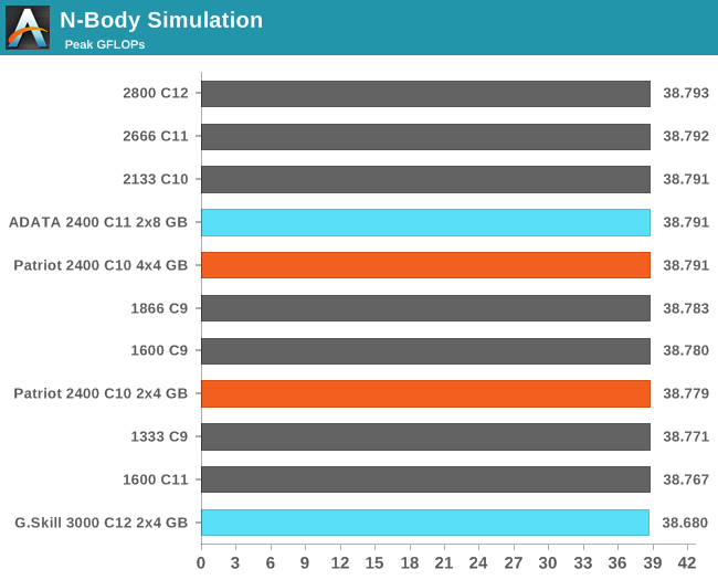
N-Body Simulation
When a series of heavy mass elements are in space, they interact with each other through the force of gravity. Thus when a star cluster forms, the interaction of every large mass with every other large mass defines the speed at which these elements approach each other. When dealing with millions and billions of stars on such a large scale, the movement of each of these stars can be simulated through the physical theorems that describe the interactions. The benchmark detects whether the processor is SSE2 or SSE4 capable, and implements the relative code. We run a simulation of 10240 particles of equal mass - the output for this code is in terms of GFLOPs, and the result recorded was the peak GFLOPs value.
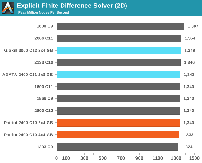
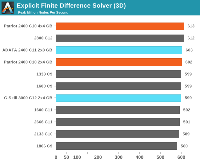
Grid Solvers - Explicit Finite Difference
For any grid of regular nodes, the simplest way to calculate the next time step is to use the values of those around it. This makes for easy mathematics and parallel simulation, as each node calculated is only dependent on the previous time step, not the nodes around it on the current calculated time step. By choosing a regular grid, we reduce the levels of memory access required for irregular grids. We test both 2D and 3D explicit finite difference simulations with 2n nodes in each dimension, using OpenMP as the threading operator in single precision. The grid is isotropic and the boundary conditions are sinks. We iterate through a series of grid sizes, and results are shown in terms of ‘million nodes per second’ where the peak value is given in the results – higher is better.
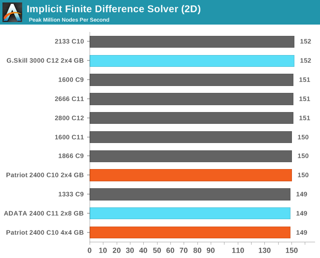
Grid Solvers - Implicit Finite Difference + Alternating Direction Implicit Method
The implicit method takes a different approach to the explicit method – instead of considering one unknown in the new time step to be calculated from known elements in the previous time step, we consider that an old point can influence several new points by way of simultaneous equations. This adds to the complexity of the simulation – the grid of nodes is solved as a series of rows and columns rather than points, reducing the parallel nature of the simulation by a dimension and drastically increasing the memory requirements of each thread. The upside, as noted above, is the less stringent stability rules related to time steps and grid spacing. For this we simulate a 2D grid of 2n nodes in each dimension, using OpenMP in single precision. Again our grid is isotropic with the boundaries acting as sinks. We iterate through a series of grid sizes, and results are shown in terms of ‘million nodes per second’ where the peak value is given in the results – higher is better.


48 Comments
View All Comments
julandorid - Monday, November 18, 2013 - link
Thanks for the review, but what exactly "featured review" means?IanCutress - Monday, November 18, 2013 - link
That's a little tagline we can attach to the front page articles when they're on the top.Wall Street - Monday, November 18, 2013 - link
I think that it is the opposite of capsule review. A featured review is a.k.a. a full review.TemjinGold - Monday, November 18, 2013 - link
Whoa... why is the 2X4 by GSkill $520?IanCutress - Monday, November 18, 2013 - link
DDR-3000 C12: you have to bin a lot of ICs to get ones with the right voltage/performance characteristics for that kit. Same reason why the more expensive CPUs are also the faster (in MHz numbers or cores) than the cheaper ones.ShieTar - Tuesday, November 19, 2013 - link
True. But you can get DDR 2666 with CL10 for about 100€, so a set with an 7% shorter access time (higher "PI" as Ian insists on calling it), and only a 11% lower transfer rate for about a fifth of the price.The 500$ kit seems to be exclusively for those who don't have to work for their money, or maybe those who are hunting records as a hobby.
DanNeely - Tuesday, November 19, 2013 - link
The very top of the line always is extremely expensive, and - when it's the result of extreme binning - has to be in order to limit demand to the miniscule supply available.Gen-An - Tuesday, November 19, 2013 - link
Exactly, they have to test the ICs individually with those tester kits and bin them for speed. I just find it amazing that a chip that is designed for say, 1600 C11 at 1.5v has the potential to run 3100 C12 with 1.65v, that's nearly double its rated clock speed with a mere 0.15v bump in voltage.sf101 - Monday, December 9, 2013 - link
If you want 2400 guaranteed out of the box you pay the premiums.most of the 2133 mhz black momba sticks could also do 2666mhz @ 10-13-10-30-2t but your voltages may vary.
And more than likely some of that is because of individual IMC tolerances per cpu.
Franzen4Real - Monday, November 18, 2013 - link
When it comes to memory, over the years I have tried to read up on different reviews and look at benchmarks in an attempt to understand when it is better to run tighter timings/lower MHz as opposed to looser timings/higher bandwidth. I'm sure it is a case by case basis, but was wondering if the always knowledgeable and helpful Anandtech commenters could give me a quick, dummy terms, explanation of when tight timings or clockspeed is better? Looking at your graph, it shows the C7 1866 through C10 2666 all having the same performance index score, but what situations do those different timings/MHz become better/worse? I hope this isn't too in depth of a question.I don't know if this analogy is correct, but I'm seeing it as if RAM was a race car on a track, high bandwidth/loose timings would mean your car travels faster, but has to do more laps around the track to complete. Tight timings/lower bandwidth means the car travels slower but doesn't have to do as many laps to complete. If I am correct on this, at what point does less laps trump traveling faster?
As a side note, I am looking to build a Haswell desktop in Jan/Feb. It will have one GPU (probably one of the R9's) and more than likely a 2x8gb RAM kit. My usage would very roughly be 70% gaming, 25% rendering in 3DS Max and using some Adobe programs, 5% or less video encoding. I'm looking for help in deciding what to look for in this scenario, but also to finally have a better understanding of how these settings affect different workloads.
Sorry for the wall of text!!